
A Reconciled Attribution Chart Is Not Proof of Alpha
Accounting identities, factor regressions and investment skill are different claims. Two synthetic examples show what reconciliation proves, how scaling changes attribution, and why a fitted residual is not evidence of alpha.
A waterfall chart has an unfair advantage in a research presentation: it looks like an explanation. There is the market contribution, there are a few other factors, there is a residual, and the bars add up to the observed result. The arithmetic feels reassuringly complete.
It should be reassuring about the arithmetic. It should not, by itself, be reassuring about investment skill. Accounting reconciliation, statistical explanation and evidence of alpha are three different claims. A chart can succeed at the first, be conditional on debatable choices at the second, and say very little about the third.
The way to make attribution useful is not to abandon it. It is to give each layer a precise job, with the right units, endpoints and tests. We will start with a small ledger whose answer can be checked by hand, then move to a separate synthetic regression example.
First, make the money add up
Suppose a fictional account opens with 10 shares marked at $100 and $1,000 in cash. Its opening equity is $2,000. During the period it buys four shares at $102, paying a $1 fee, then sells three at $105, paying another $1 fee. At the end, the asset is marked at $104.
Assume no external deposits or withdrawals, dividends, financing costs, foreign exchange changes or corporate actions. Every amount is in one currency. There is no ambiguity about the two executions in this example.
| Event | Quantity change | Price | Fee | Cash after | Shares after |
|---|---|---|---|---|---|
| Opening state | — | $100 | — | $1,000 | 10 |
| Buy | +4 | $102 | $1 | $591 | 14 |
| Sell | −3 | $105 | $1 | $905 | 11 |
| Closing mark | 0 | $104 | $0 | $905 | 11 |
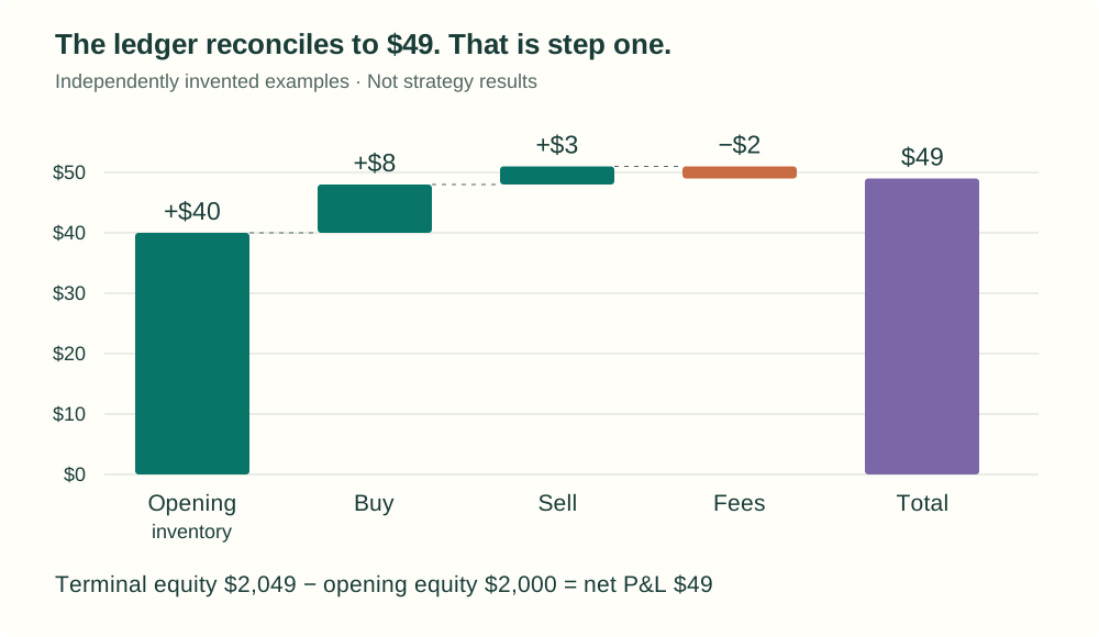
Closing equity is $905 plus 11 × $104, or $2,049. Net P&L is therefore $49. We can independently express that result as a bridge from opening inventory and subsequent executions to the closing mark:
Buy contribution: 4 × (104 − 102) = $8
Sell contribution: −3 × (104 − 105) = $3
Fees: −$2
Net P&L: $40 + $8 + $3 − $2 = $49
In general, for this single-asset, self-financing setup, let signed quantity changes be positive for buys and negative for sells:
+ Σj Δqj(PT− Pj) − Σj feej
This is one valid decomposition of marked wealth, not the only possible accounting presentation. A realised/unrealised split additionally needs an inventory cost-basis convention. External cash flows, dividends, financing, currency translation and corporate actions need their own consistent treatment before extending the identity to a real account.
The accounting layer should reconcile without knowing anything about a factor model. If it does not, a regression should not be allowed to absorb the mismatch into an impressive-looking “unexplained” bar.
A dollar sensitivity is not a portfolio beta
Now introduce a statistical model across periods. Let yt be monetary P&L and fkt be a factor return, represented as a decimal: 1% is 0.01. A linear decomposition is:
Here a, each contribution and the residual are in currency. A coefficient of 500 means a one-percentage-point factor move contributes $5 in the fitted model, holding other included factors fixed. It is not a dimensionless beta of 500, nor proof that $500 was literally invested in a tradable factor portfolio.
To discuss return betas, first define portfolio returns and their capital denominator. Changing capital, intraperiod cash flows and leverage make that a substantive measurement choice. Dividing every period's P&L by an arbitrary constant may make a chart look like a return series; it does not automatically make it the desired economic return.
Timing is just as important as units. If the portfolio outcome covers one interval and the factors cover another, the residual includes that mismatch. Split and reconcile the outcome at common endpoints before interpreting exposures. A better fit obtained by shifting an endpoint after looking at the results also belongs in the research history.
Standardisation changes the coordinates, including the intercept
Correlated factors can make ordinary least-squares coefficients unstable. Ridge regularisation is one way to trade some fit for coefficient shrinkage. It does not remove the need to specify the factors, and its penalty depends on how their coordinates are scaled.
Suppose each training factor is standardised using training mean μk and a strictly positive training scale sk. Fit a model in those coordinates:
ŷt = az+ Σk θkzkt
Minimise Σt(yt − ŷt)2 + λΣkθk2
The intercept is unpenalised. This objective uses a sum of squared errors, not a mean; the same numerical penalty has a different meaning if that convention changes. Substituting the definition of z gives the coefficients in raw factor coordinates:
a = az − Σkβkμk
Rescaling coefficients but forgetting the intercept adjustment changes every prediction. Multiplying standardised coefficients directly by raw factor returns produces a different mistake. A zero-variance training column needs explicit handling—for this example, drop it—rather than division by zero. Freeze both means and scales when applying a fitted model to later observations.
A complete six-period example
The following is a separate, independently invented dataset, not a return history generated by the $49 ledger. Its two anonymous factors have no connection to a real portfolio or factor family. Six rows are enough to check the algebra; they are not enough to make an investment inference.
| Period | Factor F1 | Factor F2 | P&L |
|---|---|---|---|
| 1 | −2.00% | −1.80% | −$18 |
| 2 | −1.00% | −0.70% | −$12 |
| 3 | 0.00% | −0.20% | $3 |
| 4 | 1.00% | 1.40% | $16 |
| 5 | 2.00% | 1.60% | $17 |
| 6 | 3.00% | 3.10% | $34 |
Download the invented regression inputs (CSV). Factor returns in the download are decimals, not percentage points.
Use all six rows for this deliberately in-sample arithmetic check. With population standard deviations (divisor six), the factor means are 0.005 and approximately 0.005667; their scales are approximately 0.017078 and 0.016316. At λ = 2 under the stated sum-of-squares objective, the standardised coefficients are approximately 7.5002 and 7.6665, with an intercept of 6.6667.
The raw-coordinate model has an intercept of approximately $1.8083 and coefficients of 439.1669 and 469.8649 currency units per unit factor return. For period 6, the fitted contributions are:
F1: 439.1669 × 0.03 ≈ $13.1750
F2: 469.8649 × 0.031 ≈ $14.5658
Residual: $4.4509
Total: $34.0000
The displayed numbers are rounded; calculations use full precision. If we mistakenly kept the standardised intercept of 6.6667 alongside the raw coefficients, predictions would be shifted upward by about $4.8584 in every period. An independent prediction-equivalence check catches that error before it reaches a report.
Several explanations can all reconcile
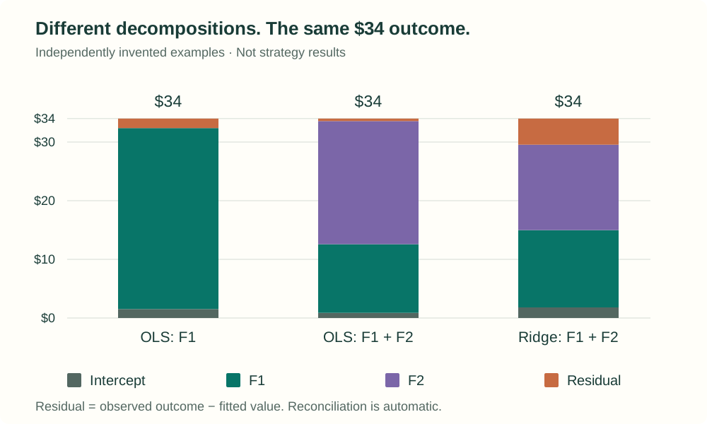
Fit the same six outcomes with one factor, with both factors, or with standardised ridge. The contributions change. The observed P&L does not. Define the residual as outcome minus fitted value and every model reconciles by construction.
| Model | Intercept | F1 | F2 | Residual | Total |
|---|---|---|---|---|---|
| OLS: F1 only | 1.5238 | 30.8571 | — | 1.6190 | 34.0000 |
| OLS: F1 + F2 | 0.8787 | 11.6979 | 20.9977 | 0.4256 | 34.0000 |
| Ridge: F1 + F2 | 1.8083 | 13.1750 | 14.5658 | 4.4509 | 34.0000 |
Independently rounded cells can differ slightly from the displayed total. The unrounded quantities reconcile. More importantly, neither reconciliation nor in-sample fit decides which specification captures the relevant economics. Factors are measurements with construction choices, not self-evident explanations. Even a familiar public factor family has a defined universe, weighting rule and return convention; the Fama/French construction notes are a useful reminder of that specificity.
A zero-mean residual is often a first-order condition
In an unweighted least-squares or ridge fit with a freely fitted, unpenalised intercept, differentiating the objective with respect to that intercept gives:
Up to numerical tolerance, the training residuals sum to zero. Their individual values can still be large. This is a property of the fit, not evidence that no economically unexplained profit remains. Weighted fitting gives a weighted condition; constrained or penalised intercepts change the argument. It also does not force future residuals to average to zero.
Calling the fitted intercept “alpha” does not supply the assumptions needed to interpret it as skill. In our P&L regression it is a currency intercept, not automatically risk-adjusted excess return. It can reflect omitted exposures, nonlinear relationships, valuation mismatches, changing capital, costs, sample selection or instability. Those are questions for the research design, not defects repaired by renaming a chart label.
Regularisation adds another model choice. Shrinking factor slopes can reallocate the fitted explanation between slopes and intercept. The shift from the two-factor OLS intercept to the ridge intercept above happens without generating a cent of additional P&L. It would be a mistake to rank those intercepts as competing estimates of newly discovered skill without examining the model and evaluation contract.
Held-out reconstruction is not necessarily an advance forecast
A sensible validation can fit exposures only on earlier periods and apply them to a later period. That tests something useful: how well an estimated relationship carries forward. But ask which inputs the reconstruction uses.
If the factors on the right are the returns realised during period t, the result is a held-out conditional reconstruction. It is not a forecast that was available before the period started. The coefficients may be properly lagged while a critical input still belongs to the future at the putative decision time.
An advance forecast needs factor forecasts or another admissible information set, with the additional uncertainty that implies. A trading claim also needs a feasible policy and costs. Neither follows from a low held-out reconstruction error.
Uncertainty around exposures or an intercept should respect dependence and the actual sampling unit. Model selection, repeated specification changes and changing portfolio composition matter too. Six invented rows cannot answer those questions, which is why this example reports arithmetic rather than a significance claim.
A useful claim ladder
- Accounting: executions, inventory, cash and marks reconcile, with fees and other flows accounted for once.
- Statistical explanation: contributions are correct under a stated model, scale convention, factor set and time window.
- Predictive evidence: a defined forecasting procedure is evaluated using information actually available at prediction time.
- Investment-skill evidence: the economic benchmark, uncertainty, selection process and implementability support the stronger interpretation.
Each step needs evidence that the preceding step does not provide. For the first two, useful acceptance checks are pleasantly concrete: rebuild terminal wealth independently of the bridge; reverse the sign of a trade in a controlled fixture; ensure fees enter once; match endpoints; compare standardised and raw-coordinate predictions; and verify the residual condition only where its assumptions apply.
These checks are not cosmetic. They keep implementation errors from masquerading as economics. Once they pass, however, the harder questions about the model and the investment claim still remain.
Reconciliation is the floor for attribution, not the ceiling of the research. A chart earns trust by stating what it explains, how it was calculated and what would be needed to make a stronger claim—not by making its residual disappear.
Further reading
- Scikit-learn: linear models and ridge regression. The documented penalised sum-of-squares objective is the convention used in the synthetic example; the coordinate transformation is derived above.
- Kenneth French: description of Fama/French factors. An original source for a specific public factor construction—not an endorsement of those factors for every portfolio.
- Mitchell Petersen: Estimating Standard Errors in Finance Panel Data Sets. Background on dependence-aware inference. The working paper compares methods under particular data structures; it does not make one standard-error choice universally correct.