
Before You Call It a Failed Replication
A published anomaly earns 12.3% a year over sixty years of US data; seven years of Australian data give a t-statistic of 1.0. What a short sample can say, how microstructure can fake a result, and a protocol that makes either answer informative.
The simulations in this article use invented parameters. The Australian figures in “What our own test showed” come from our own historical backtest: they are not a trading record and not evidence of achievable returns.
On Australian data from 2019 to 2025 — 83 months — our value-weighted version of the strategy returned 0.54% a month, with a t-statistic of 0.99. The tempting headline is "doesn't work in Australia".
But run the numbers. Our long-short portfolio's volatility was about 5% a month. At that volatility, even if the effect were exactly as large in Australia as in the US, seven years of data would give an expected t-statistic of only 1.9, and we would miss the effect more often than we found it (power 47%). Our observed t of 0.99 is almost exactly as likely if the effect is real as if it is absent: the likelihood ratio is 1.08. We had run a coin-flip, and nearly reported it as a verdict.
The opposite mistake is just as easy. Some signals built from daily price data can be manufactured by the mechanics of how closing prices are recorded. A small, thinly traded market is where that mechanism is strongest. A replication that "works" can be as uninformative as one that "fails".
This article works through both problems, using our own test as the example, and ends with the protocol we now use when porting a published anomaly to a new market.
Three studies, three verdicts
Whether published stock-return anomalies replicate is a question three large studies answer very differently, and the gap between them is the most useful lesson for anyone working in a small market.
Hou, Xue and Zhang (2020) rebuilt 452 anomalies from the literature. They sorted US stocks into deciles using NYSE breakpoints and value-weighted returns, to stop tiny stocks from dominating. They then asked whether each long-short return cleared the conventional |t| ≥ 1.96. Only 158 did: 65% failed. Raising the bar to 2.78 to allow for multiple testing, 82% failed. When they weighted stocks equally instead, which lets small stocks back in, the success rate rose to about 56–59%.
For the kind of signal in our worked example, one category matters most. Among "trading frictions" anomalies — built from recent daily trading behaviour, such as a stock's maximum daily return last month — 96% failed. Weighting towards small stocks did not rescue the category. A signal built from the signs of last month's daily returns is a close cousin of that family. So the published prior for this kind of result is not "most anomalies are shaky" but "almost all of this type are".
Jensen, Kelly and Pedersen (2023) start from the same question and reach the opposite conclusion. Their baseline on US data is a 55.6% replication rate. It is higher than Hou–Xue–Zhang's 35% because of a longer sample and different portfolio construction: tercile rather than decile spreads, breakpoints from non-micro stocks, and capped value weights. They test risk-adjusted rather than raw returns. After a Benjamini–Yekutieli multiple-testing correction they report 75.6%. Under their preferred model, a hierarchical empirical-Bayes framework that lets each factor borrow strength from related factors, the US replication rate is 82.4%. Outside the US, they report lower raw replication rates "primarily due to the fact that foreign markets have shorter time samples". The estimated alphas themselves are similar in size.
Jacobs and Müller (2020) examine 241 anomalies across 39 markets. They find the United States is "the only country with a reliable post-publication decline in long-short returns". In the US, McLean and Pontiff (2016) had measured returns 26% lower out of sample and 58% lower after publication, attributing about 32 percentage points to investors trading on the published research.
These studies are not contradicting each other about the data. They are answering different questions:
- Hou–Xue–Zhang ask whether each anomaly, taken alone and judged by a fixed hurdle, survives realistic construction.
- Jensen–Kelly–Pedersen ask what we should believe about each factor given everything we know about all of them.
- Jacobs–Müller ask whether publication itself erodes returns, and find it does so reliably only where arbitrage capital is deepest.
For a researcher with seven or ten years of data from a small market, this settles the right question. Judging a local result alone against a fixed hurdle is a test the data cannot pass, and failing it proves nothing. The only question a short sample can answer is how much it should move the evidence you already had. Michael Clemens (2017) gives the vocabulary: testing a US finding on Australian data is not a replication at all but an extension, a test of whether a result generalises. A null extension is not a failed replication.
The arithmetic of a short sample
Take the worked example. Fattinger, Hanspal, Koval and Steshkova (2026) report that stocks whose recent daily returns have been mostly negative outperform stocks whose daily returns have been mostly positive. They measure this with the imbalance between up days and down days over the prior month. A long-short strategy earns 12.3% a year from 1963 to 2023.
The psychological motivation comes from Fisher and Keil (2018), who show that people often summarise graded evidence by counting how many items fall on each side of a midpoint, ignoring their size.
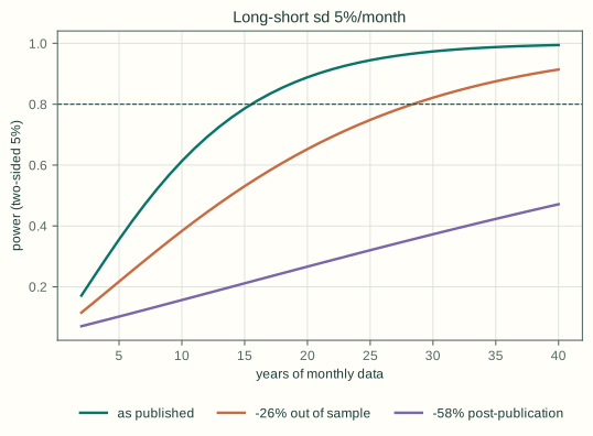
12.3% a year is about 1.03% a month. How reliably a new test can detect that depends on the volatility of the long-short portfolio, so take three illustrative levels:
- 3.6% a month, low enough that sixty years of data would give a t-statistic near 7.6;
- 5%, close to our own;
- 7%, for a thinner market.
The expected t-statistic of a new test follows directly:
| Long-short volatility | True effect | 7 years | 10 years | 20 years |
|---|---|---|---|---|
| 3.6% | 1.03% (as published) | t 2.6 · power 74% | t 3.1 · 87% | t 4.4 · 99% |
| 3.6% | 0.76% (−26% out of sample) | t 1.9 · 48% | t 2.3 · 63% | t 3.2 · 90% |
| 3.6% | 0.43% (−58% post-publication) | t 1.1 · 19% | t 1.3 · 26% | t 1.8 · 45% |
| 5.0% | 1.03% | t 1.9 · 47% | t 2.2 · 61% | t 3.2 · 89% |
| 7.0% | 1.03% | t 1.3 · 27% | t 1.6 · 36% | t 2.3 · 62% |
Power of a two-sided 5% test. Haircuts from McLean and Pontiff (2016).
Flip the question round, and the smallest effect seven years of data can reliably detect (80% power) is 1.1% a month at 3.6% volatility. At 5% volatility it is 1.5%, and at 7% it is 2.1%. All of these are larger than the published effect. To detect the published effect at 5% volatility you need about 15 years of data. To detect the post-publication version you need about 88.
Why small-market portfolios are noisier
The 5% and 7% rows are not arbitrary: our own long-short volatility was about 5% a month. Those rows follow from how concentrated small markets are.
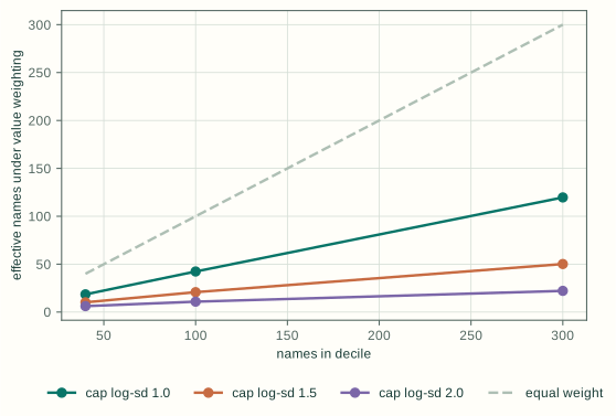
Value weighting is the right economic choice: it reflects what investors can actually hold, and Hou, Xue and Zhang are right to insist on it. But in a market where a handful of companies are very large, a value-weighted decile of 40 stocks does not diversify like 40 stocks. The effective number of holdings, 1/Σw², collapses as company sizes spread out:
| Spread of company sizes (log sd) | 40 names per decile | 100 names | 300 names |
|---|---|---|---|
| 1.0 | 18.5 effective | 42.4 | 119.7 |
| 1.5 | 10.2 | 20.8 | 50.2 |
| 2.0 | 6.2 | 10.9 | 22.2 |
Median across 2,000 simulated deciles with lognormal market capitalisations.
With a typical stock's specific risk at 10% a month, a long-short portfolio holding six effective names on each side has a volatility of about 6.4% a month. With twenty on each side it is about 4.3%. That is the whole difference between a test that can see an effect and one that cannot. Report both value-weighted and equal-weighted results, and decide in advance which one the conclusion rests on.
How to read a weak result
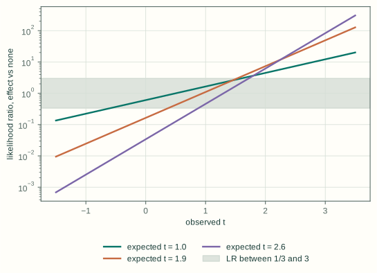
"Not significant" is not a finding. The informative number is how much more likely the observed result is if the effect is real than if it is not. If the effect would produce an expected t-statistic of δ, the likelihood ratio for an observed t is exp(t·δ − δ²/2):
| Expected t if the effect is real | observed t = −1 | 0 | 1 | 2 | 3 |
|---|---|---|---|---|---|
| 1.0 | 0.22 | 0.61 | 1.65 | 4.48 | 12.2 |
| 1.9 (our sample: seven years, 5% volatility) | 0.03 | 0.16 | 1.10 | 7.35 | 49.2 |
| 2.6 | 0.00 | 0.03 | 0.46 | 6.17 | 83.1 |
With our seven years, an observed t of about 1 moves the odds by about 10%. It is not evidence. By contrast, an observed t of zero would have been meaningful evidence against the full effect (a ratio of 0.16, about 6 to 1), and a t of 2 strong evidence for it.
Campbell Harvey's (2017) minimum Bayes factor makes the same point from the other side. Even a t of 2 leaves more room for the null than a p-value of 5% suggests. That is part of why Harvey, Liu and Zhu (2016) argue new factors should clear t > 3.
The practical method is to combine, not to replace. Start from a prior for the local effect: the published estimate, cut for post-publication decay and uncertainty about whether it transfers across markets. Update it with the local estimate:
posterior mean = (μ_prior/τ² + μ̂/se²) / (1/τ² + 1/se²)
Jensen, Kelly and Pedersen's hierarchical model is the full version of this idea, pooling across factors and countries. With a short local sample, the posterior will sit close to the prior unless the local evidence is very strong. That is the honest answer, not a failure of the method.
What our own test showed
On ASX data from 2019 to 2025, our value-weighted decile long-short version of the signal returned 0.54% a month (Newey–West t = 0.99, 83 monthly returns). Its 95% interval runs from −0.53% to +1.60%, which contains the published 1.03%. The point estimate has the published sign.
Here is what that result can and cannot say about each version of the published effect:
| Effect we might expect | Expected t in our sample | Power | Likelihood ratio at our t, effect vs none |
|---|---|---|---|
| 1.03% a month (as published) | 1.89 | 47% | 1.08 |
| 0.76% (−26%, the out-of-sample decline) | 1.40 | 29% | 1.50 |
| 0.43% (−58%, the post-publication decline) | 0.79 | 13% | 1.60 |
No row moves the odds by more than 60%. The data lean very slightly toward a positive effect smaller than the published one, and barely distinguish it from no effect at all.
Now apply the posterior formula. Take a prior centred on the US estimate cut by 26% for data mining — Jacobs and Müller find no reliable post-publication decay outside the US — so 0.76% a month, with a standard deviation of 0.5% for uncertainty about whether the effect transfers across markets. Our seven years move that to 0.66% ± 0.37%. The estimate shifted by a tenth of a percent a month, and the uncertainty narrowed by about a quarter. That is what seven years of a small market can tell you about a 1%-a-month effect.
Before reading anything into the point estimate, the checks in the next section come first. We have not yet run the microstructure placebos on this sample; the result is too weak to need them for its verdict, but not for its interpretation.
The part that can fake it
Short samples make real effects hard to see. The microstructure of a small exchange can make an effect appear where none exists. Signals built from daily signs are especially exposed, and it helps to know why.
Zero-return days. A sign-based signal scores days with no price change as zero. In thinly traded stocks those days are common: Lesmond, Ogden and Trzcinka (1999) turned the frequency of zero-return days into a measure of trading costs. How to treat them is a real design choice. Da, Gurun and Warachka (2014) define a related sign-count measure, "information discreteness", with zero days in the denominator. They also define an alternative that normalises only over days with non-zero returns. In our simulations below the choice barely matters (0.61% versus 0.59% a month with half of all days stale), but it should be stated, not assumed.
Tick size. On the ASX, prices move in steps of 0.1¢ below 10¢, 0.5¢ from 10¢ up to $2.00, and 1¢ from $2.00. One tick is 2.5% of the price of a 20¢ stock, 0.33% at $1.50 and 0.02% at $50. Discrete prices make daily signs lumpy at low prices, and a price floor calibrated to US tick sizes does not remove this.
The closing print. The larger issue is where the "close" comes from. If a stock's last trade of the day is at the bid, the close sits below fair value, that day's return looks negative, and the next day's return will tend to bounce back up. Any signal that counts recent up and down days is exposed to this. How exposed depends on how much weight it puts on the final days of the formation window.
Here is a worked example of our own, not the paper's specification. Weight each day by exp(λ·(j−1)), where j counts trading days through the month, so recent days count more. With λ = 0.13, a 21-day month puts about 13% of the signal on the last day and about 35% on the last three. With every day weighted equally, the last day still carries 4.8%. A bid close on the last day of the month pushes the stock toward the "mostly down" end of the ranking, which is the end the strategy buys. The first day of the holding month then includes the bounce back to fair value. That is exactly the direction of the published effect.
To measure how much this matters, we simulated 1,000 stocks for ten years in a world with no true effect at all. Prices wander randomly with no drift, and each day's close prints at the bid or the ask at random. Each month we formed the λ = 0.13 sign signal, bought the lowest decile and sold the highest. We then repeated the test with three remedies:
| Half-spread | Baseline | Drop last day from signal | Skip one day before holding | Hold from midquote |
|---|---|---|---|---|
| 0.00% | +0.02% | −0.00% | +0.01% | +0.02% |
| 0.50% | +0.15% (t 1.3) | −0.01% | −0.01% | −0.01% |
| 1.00% | +0.60% (t 5.0, significant in all 50 runs) | −0.02% | −0.02% | −0.02% |
| 2.00% | +2.01% (t 16.5) | −0.01% | +0.00% | +0.01% |
Low-minus-high monthly return, averaged over 50 simulations of 1,000 stocks × 120 months. Equal-weighted deciles.
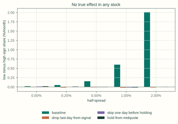
At a 1% half-spread, which is unremarkable for a small-cap stock, the no-effect world produces about 0.6% a month, significant in all 50 simulations. Any one of three small changes removes it:
- dropping the last day from the signal;
- leaving a one-day gap between forming the portfolio and holding it, a standard check in the short-term reversal literature (Jegadeesh 1990; Lehmann 1990);
- measuring holding-period returns from midquotes.
The spurious spread scales with the weight on the final day, and it does not disappear when every day is weighted equally:
| Weight on the last day of the month | Null-world spread at 1% half-spread |
|---|---|
| 4.8% (all days equal, λ = 0) | +0.28% (t 2.3; significant in 70% of runs) |
| 8.5% (λ = 0.065) | +0.48% (t 3.8) |
| 13.0% (λ = 0.13) | +0.60% (t 5.0) |
| 18.4% (λ = 0.2) | +0.70% (t 5.8) |
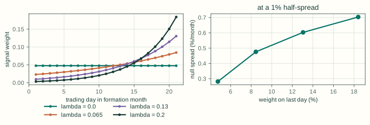
This dose-response gives a check anyone can run on any recency-weighted signal, whatever its exact specification. Compute the equal-weighted version of the same signal and report it beside the weighted one. If the result is genuinely about the imbalance of up and down days, the two versions should broadly agree. If they disagree — the equal-weighted version is much weaker, or flips sign — then the result is carried by the weighting scheme, and the weighting, not the behavioural story, is what needs explaining. Month-end microstructure is the first suspect.
We are not claiming the published US result is caused by bounce. Value weighting, the paper's own checks and the much tighter spreads of large US stocks all work against it, and the paper's exact weighting scheme is its own. The point is that these checks cost a line of code each, and a local test is most exposed exactly where the signal is strongest: in thin stocks with wide spreads.
On the ASX there is a further wrinkle. Most closing prices are set by a closing auction, where all orders match at one price rather than at the bid or ask. But when buy and sell orders do not overlap before that auction, the ASX takes the close from the last trade in normal trading. Bounce exposure therefore concentrates in the least liquid names. Flag every close by its source.
Data traps that a small exchange amplifies
- Delistings. Shumway (1997) found that missing delisting returns for companies removed for poor performance averaged about −30%. Data panels that quietly drop dead companies overstate the returns of exactly the stocks that sort into "losers". Count how many delisted companies your panel keeps before trusting anything.
- Identity. A ticker is a listing identifier with effective dates, not a permanent identity. Key the panel on a point-in-time security master, with dated code and name histories, never on the ticker string.
- Corporate actions. Share consolidations are common among small companies, and an unadjusted consolidation day is a large false sign. Ex-dividend drops are larger and more predictable where dividends carry franking credits. Use adjusted returns for signs, and audit the adjustments.
- Local factors. Build risk controls from the local market's own data, as Brailsford, Gaunt and O'Brien (2012) do for Australia. State plainly which of the original paper's controls you cannot rebuild.
Can anyone trade it?
A one-month signal with little persistence from month to month turns over almost completely. In our no-effect simulation, 90% of each decile changed every month, exactly what independent rankings imply.
Novy-Marx and Velikov (2016) find that most anomalies with one-sided monthly turnover below about 50% stay significant after costs, and few above that level do. They also find that a buy/hold band — buy on a strong signal, sell only on a weak one — is the most effective simple way to cut costs. Chen and Velikov (2023) put the average anomaly's expected return, net of spreads and post-publication decay, at about 4 basis points a month, and no more than 10 for the strongest.
In a small market, add borrow constraints: the stocks the short side wants are often the hardest to borrow.
The protocol
Before running the test:
- Name the estimand and the expected effect, including an explicit haircut from the published estimate.
- Compute power and the minimum detectable effect for your sample length, at both value and equal weights. If power is below 50%, the only honest write-up is "consistent / inconsistent with an effect of size δ", never "fails to replicate".
- Audit the construct. Report the share of zero-return days, tick-size exposure and the weight on the last days of the formation window, by decile.
- Report the equal-weighted version beside any recency-weighted version, and treat disagreement between them as a finding about the weighting.
- Run the microstructure placebos: skip a day, hold from midquotes or auction prices, and flag every closing price by source.
- Check data integrity: delisted-company coverage, identifier continuity and corporate-action adjustments.
- Separate the signal from its neighbours: short-term reversal and existing sign-count measures.
- Test implementation: returns net of costs, with borrow-feasible short legs.
When reporting:
- Give the likelihood ratio or posterior and the decision it supports, not a lone t-statistic.
What this does not show
Our own test cannot say whether the anomaly exists in Australia, and nothing else here can either. The power calculations use the published US headline, our realised volatility and illustrative alternatives. The bounce simulation shows that a no-effect world can produce the published sign pattern, not that it does in any real sample.
What the arithmetic does show is that a short, thin market can rarely reject a published effect, and can sometimes manufacture one. A replication worth reporting is designed so that both mistakes are visible before the result is known.
References
- Brailsford, T., Gaunt, C., and O'Brien, M. A. (2012). Size and book-to-market factors in Australia. Australian Journal of Management 37(2), 261–281.
- Chen, A. Y., and Velikov, M. (2023). Zeroing in on the expected returns of anomalies. Journal of Financial and Quantitative Analysis 58(3), 968–1004.
- Clemens, M. A. (2017). The meaning of failed replications: a review and proposal. Journal of Economic Surveys 31(1), 326–342.
- Da, Z., Gurun, U. G., and Warachka, M. (2014). Frog in the pan: continuous information and momentum. Review of Financial Studies 27(7).
- Fattinger, F., Hanspal, T., Koval, B., and Steshkova, A. (2026). Binary bias and stock returns. SSRN Working Paper 7460480.
- Fisher, M., and Keil, F. C. (2018). The binary bias: a systematic distortion in the integration of information. Psychological Science 29(11), 1846–1858.
- Harvey, C. R. (2017). Presidential address: the scientific outlook in financial economics. Journal of Finance 72(4), 1399–1440.
- Harvey, C. R., Liu, Y., and Zhu, H. (2016). …and the cross-section of expected returns. Review of Financial Studies 29(1), 5–68.
- Hou, K., Xue, C., and Zhang, L. (2020). Replicating anomalies. Review of Financial Studies 33(5), 2019–2133.
- Jacobs, H., and Müller, S. (2020). Anomalies across the globe: once public, no longer existent? Journal of Financial Economics 135(1), 213–230.
- Jegadeesh, N. (1990). Evidence of predictable behavior of security returns. Journal of Finance 45(3), 881–898.
- Jensen, T. I., Kelly, B., and Pedersen, L. H. (2023). Is there a replication crisis in finance? Journal of Finance 78(5), 2465–2518.
- Lehmann, B. N. (1990). Fads, martingales, and market efficiency. Quarterly Journal of Economics 105(1), 1–28.
- Lesmond, D. A., Ogden, J. P., and Trzcinka, C. A. (1999). A new estimate of transaction costs. Review of Financial Studies 12(5), 1113–1141.
- McLean, R. D., and Pontiff, J. (2016). Does academic research destroy stock return predictability? Journal of Finance 71(1), 5–32.
- Novy-Marx, R., and Velikov, M. (2016). A taxonomy of anomalies and their trading costs. Review of Financial Studies 29(1), 104–147.
- Shumway, T. (1997). The delisting bias in CRSP data. Journal of Finance 52(1), 327–340.
- ASX. Australian equities trading (price steps) and Auctions (closing price determination). asx.com.au, accessed September 2026.