
The Half-Life of What? Signal Decay Is Not the Cost of Waiting
The same price path can produce several different decay curves. A worked example separates marked returns, delayed entry and hindsight opportunity—and explains what a decision-relevant cost of waiting must specify.
A half-life is a wonderfully compact answer to a question that has often not been specified. “The signal has a half-life of ten minutes” sounds operationally useful. But what halves? An expected return? The fraction of an eventual price move still ahead? A retrospectively measured opportunity? Or the effectiveness of the model as other participants learn the same trick?
These are different objects. They can move in different directions, and they do not automatically answer the practical question: what do we give up by waiting before acting? The distinction matters before any curve fitting, optimisation or infrastructure decision. A more sophisticated fit cannot rescue an ambiguous target.
Here we will separate the questions using a small price path, then work back to what a decision-relevant measurement would require. There is no estimated trading signal in the example. That is deliberate: the arithmetic should be clear before we ask whether a model predicts it.
One path, several perfectly legitimate answers
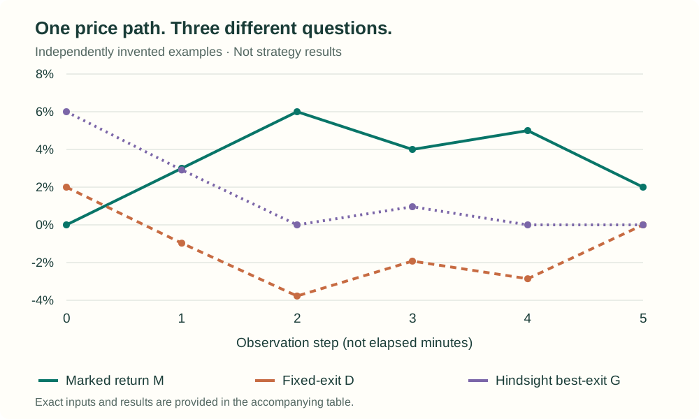
Suppose six observations of a fictional asset have prices of 100, 103, 106, 104, 105 and 102. Label the observations 0 through 5, and fix the terminal observation at 5. Choose the long direction in advance. These labels are observation steps, not minutes or trading sessions.
For now, treat the marks as frictionless transaction prices. Ignore spread, fees, market impact, financing and the possibility of not being filled. This is an arithmetic example, not a claim that those assumptions are realistic.
Write the price at observation t as Pt, the initial price as P0, and the fixed terminal observation as H. Three useful quantities are:
- Marked return since the initial entry: how far the price has moved relative to the original reference.
- Delayed-entry return to the fixed exit: what the price path would pay if entry moved to t but exit stayed at the already specified H.
- Best-future-exit return from a delayed entry: the best outcome available after t, selected with hindsight.
D(t, H) = PH / Pt − 1
G(t, H) = maxt ≤ u ≤ H (Pu / Pt − 1)
These equations use decimal returns. The table and chart display percentages. The best-exit set includes u = t, so the last quantity cannot be negative in this frictionless example: immediate exit is allowed. That convention would be inappropriate for some actual execution problems and must not be left implicit.
| Step | Price | Marked M | Fixed-exit D | Hindsight G |
|---|---|---|---|---|
| 0 | 100 | 0.00% | 2.00% | 6.00% |
| 1 | 103 | 3.00% | −0.97% | 2.91% |
| 2 | 106 | 6.00% | −3.77% | 0.00% |
| 3 | 104 | 4.00% | −1.92% | 0.96% |
| 4 | 105 | 5.00% | −2.86% | 0.00% |
| 5 | 102 | 2.00% | 0.00% | 0.00% |
Download the invented price path (CSV). The three equations reproduce every return in the table.
The reference price is doing real economic work
At observation 1, someone who entered at 100 is up 3%. Someone entering now at 103 and holding to the fixed terminal price of 102 would lose about 0.97%. Someone who could select the future peak of 106 would make about 2.91%. All three statements are correct. None can be substituted for another merely because its chart looks like a response curve.
There is a fourth quantity that is particularly easy to misread: the best future price, still measured from the original entry reference. At observations 0, 1 and 2, the future maximum is 106, so the original-reference best return remains 6%. That does not mean a new entrant can still earn 6%. By observation 2 the new entrant has no positive best-exit return left in this path.
With a fixed original reference, a future maximum over an ever-shrinking set is necessarily non-increasing. That monotonicity comes from the construction. It is not evidence that an economic forecast decays smoothly. Once entry is rebased to the current price, even the hindsight curve need not be monotone: our best-exit return rises from zero at step 2 to roughly 0.96% at step 3.
A curve can retain the original opportunity in its numerator after a later entrant has already lost the opportunity to earn it. Always state both the reference price and the exit rule.
Even the simplest cost of waiting needs a unit
The marked and fixed-exit returns satisfy a useful consistency check:
Simple percentage returns compound; they do not add. Taking “terminal return minus return already realised” is not, in general, the percentage return on a later investment. At step 1, 2% minus 3% is −1%, whereas the return from 103 to 102 is approximately −0.9709%.
We also need to say what stays fixed across the two policies. For a fixed quantity of one share, immediate entry at 100 and exit at 102 makes 2 currency units. Delayed entry at 103 and the same exit loses 1. The ex-post cost of waiting is 3 currency units, before costs and any return on idle cash.
For fixed initial cash of 100 units, with fractional shares permitted and zero interest, immediate entry earns 2 units. Waiting and investing that cash at 103 earns about −0.9709 units. The difference is approximately 2.9709, not 3. Neither convention is wrong; they compare different feasible positions.
A genuine decision comparison goes further. Waiting may change the spread paid, the available quantity, the probability of execution, other opportunities for the capital, and the information on which the later action is based. The relevant object is expected net value under specified policies, conditional on the information available when the decision is made—not the ex-post maximum of a marked price path.
This is the useful distinction between a forecast and a decision input. The multi-period trading framework described by Boyd and coauthors makes that separation explicit: expected returns, risk, trading costs and holding costs enter the decision problem, while forecast generation is a separate task. It does not make any particular decay estimate valid.
Normalisation can quietly change the question
Converting every path into a fraction of its best eventual move can make aggregation look tidy. But it introduces decisions that belong in the statistical specification, not in a plotting helper.
What happens when the normalising opportunity is zero or very small? Consider a second invented path: 100, 99, 98. Including immediate exit, the best gross opportunity from the initial reference is zero. Dividing by it is undefined. Dropping the path conditions the sample on having a favourable future excursion. That is not the same population as all events available when the original decision was made.
A very small positive denominator can give an otherwise unremarkable path enormous influence. Clipping fractions into a tidy interval may hide that influence, but it also changes the statistic. Likewise, the average of individually normalised paths is generally not the ratio of an average path to an average normaliser. Specify which population and weighting you want before choosing the convenient calculation.
Missing follow-up is another source of apparent decay. If long horizons retain only a subset of events, each point on the curve may describe a different population. Show support by horizon, explain why paths end, and distinguish an available-case curve from a fixed-cohort curve. Neither is automatically the answer to the other's question.
Only now is it meaningful to ask for a half-life
For a strictly positive exponential quantity, the definition is clean:
t½ = log(2) / k
But an empirical curve may rise initially, cross zero, rebound or never cross half its initial value. Our marked-return curve starts at zero; “half the starting marked return” is not a useful decay target. Our best-exit curve rebounds. Fitting a monotone exponential to either can produce a parameter, but the parameter does not erase those features.
A first half-crossing time can be a descriptive summary without an exponential model, provided the rule handles rebounds, interpolation and paths that never cross. Do not report a finite crossing just because the observation window ended. Keep an estimated crossing, a censored crossing and a fitted-model extrapolation separate.
The clock also matters. Ten observations are not ten minutes when data arrive irregularly. Ten civil minutes need not contain ten minutes of continuous trading. A volume-based clock answers another question again. Record market closures and the actual endpoints rather than silently stretching or compressing them. Our six-step example intentionally claims no conversion to a real market clock.
Finally, within-event timing is different from model performance deteriorating across months or years. The latter concerns a changing relationship between a forecast and outcomes, competition, populations or regimes. Calling both “alpha decay” does not give them a common half-life. The earlier sentiment article on this site concerns the competitive/model-generation question; this article concerns the definition of the within-event measurement.
A measurement contract before a trading rule
Before putting a decay statistic into a decision process, I would want the following questions answered in plain language:
- What is measured? Marked return, expected forward return, a hindsight opportunity or policy value?
- What is fixed? Entry reference, exit rule, quantity, capital and treatment of idle cash?
- What was knowable? Which inputs were available at the decision, and which exist only retrospectively?
- Which clock and population? Actual endpoints, eligibility, weights and follow-up coverage?
- How are awkward paths handled? Zeros, losses, small denominators, missing data and non-crossings?
- What makes the comparison executable? Costs, fills, constraints and a prespecified policy rather than a future-best exit?
The arithmetic can be checked before any empirical study. Rebase every price by the same positive constant: percentage curves should not change. At the terminal step, both delayed-entry quantities should be zero under our definitions. Calculate future maxima with a simple reference loop. Check the compounding identity. These small tests catch reference-price and endpoint mistakes that a smooth chart can conceal.
None establishes predictive value. That needs an independently evaluated forecasting or policy experiment, including uncertainty and realistic implementation assumptions. The point is to avoid giving that experiment an ambiguous target in the first place.
The useful question is not “what is the half-life?” It is “the half-life of which quantity, measured under which information and trading assumptions?” Once that is clear, the cost of waiting becomes a separate, testable decision question.
Further reading
Stephen Boyd, Enzo Busseti, Steven Diamond, Ronald Kahn, Kwangmoo Koh, Peter Nystrup and Jan Speth (2017), Multi-Period Trading via Convex Optimization, Foundations and Trends in Optimization, 3(1), 1–76. Useful background on the distinction between forecasts and cost-aware decisions. The path definitions and invented examples above are derived explicitly here, not attributed to that paper as a new decay model.
Back to all research