
Trading a Forecast, Not a Signal
“Buy” is not an instruction. A forecast curve, a liquidity profile and a cost model together determine a trading path. Three results every portfolio manager should know, and a toy optimiser that shows them.
Two forecasts both say a stock will close 10 basis points higher than it is now.
One gets there by rising steadily all day. The other jumps 35 basis points in the first hour and gives most of it back.
A signal-based system sees the same thing twice — buy — and does the same thing twice: buy at the open, sell at the close. An optimal trader buys the first gradually. The second it buys immediately, sells before the peak, and then shorts the fade. Same signal, opposite afternoons.
The gap between those two traders is where a great deal of implementation value is won or lost. This article is about how to close it.
From a signal to a forecast curve
A signal is a direction, sometimes with a strength. A forecast curve is the expected cumulative return from now to each future moment: A(t). The signal is just the sign of A at the horizon. That summary throws away when the return is expected to arrive, which is exactly what an execution decision needs.
Two strands of the literature make the point precisely.
- Gârleanu and Pedersen (2013) solve the problem of trading on return predictors with different decay speeds when trading is costly. Their answer has two principles: aim in front of the target, and trade partially toward the current aim. Persistent predictors deserve more weight than fast-decaying ones of the same strength. Because trading is expensive, you never move all the way to the target at once.
- Lehalle and Neuman (2019) show how a short-horizon signal enters an execution problem as a drift term. A forecast of rising prices makes waiting to buy more costly, and a forecast of falling prices makes it cheaper.
In both, what drives the optimal trade is the shape of expected returns over time, not their sign.
What trading actually costs
Trading costs come in three layers.
- Linear costs: half the bid-ask spread plus fees, paid on every unit traded.
- Temporary impact: the price concession for trading quickly. It rises with trading speed, but more slowly than proportionally. Almgren, Thum, Hauptmann and Li (2005), using a large institutional dataset, rejected the popular square-root form at the 95% level and settled on an exponent of 3/5. Tóth et al. (2011) document the square-root law for the total impact of large orders across markets.
- Transient impact: impact that decays after you stop trading. Obizhaeva and Wang (2013) show that when the order book replenishes at a finite speed, the optimal strategy is an initial larger trade followed by a stream of smaller ones. It depends on how fast liquidity recovers, not on the static depth of the book.
A warning belongs here. Gatheral (2010) shows that you cannot choose the shape of impact and the speed of its decay independently. Some combinations imply that a round trip has negative expected cost: a model that pays you to trade with yourself. Any cost model used for optimisation should be checked for this.
The one-trade problem, and the share of edge you keep
Start with the simplest version: buy Q shares, hold, sell. Let a be the expected edge after paying the spread and fees on both legs. Suppose the impact cost per share on each leg rises like (Q/V)^β, where V is the volume available when you trade. Expected profit is
π(Q) = a·Q − c·Q^(1+β), with c = k·σ·(V_in^−β + V_out^−β),
where σ is volatility and k is a constant. Setting the derivative to zero gives
Q = [a / ((1+β)·c)]^(1/β), and π = a·Q* · β/(1+β).
The last expression holds for any liquidity, any volatility and any edge. At the profit-maximising size, the share of the after-spread edge you keep is β/(1+β). Impact takes the rest.
| Impact exponent β | Share of after-spread edge kept | Size multiplier if the exit is impact-free | Size multiplier when edge doubles from 40 to 80 bps |
|---|---|---|---|
| 1/2 (square-root law) | 1/3 | 4.0× | 5.4× |
| 3/5 (Almgren et al. 2005) | 3/8 | 3.2× | 4.1× |
| 1 (linear impact) | 1/2 | 2.0× | 2.3× |
Closed forms checked numerically; illustrative constants. The last column assumes 5 bps of spread and fees per side, so the after-spread edge goes from 30 to 70 bps.
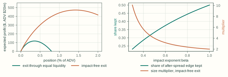
Three consequences follow.
- Most of a trade's gross edge is spent getting in and out. Under the square-root law, two-thirds of what remains after the spread goes to impact at the optimal size. If a backtest shows you keeping much more than that, it is either trading too small or its cost model is too kind.
- Exit liquidity is worth as much as entry liquidity. If the exit costs no impact — into a deep closing auction, say — optimal size rises by 2^(1/β). That is 4× under the square-root law. You price the exit before the entry.
- Size is extremely sensitive to the number you know least well. Doubling the forecast edge more than quintuples the optimal position under the square-root law. The after-spread edge is the most uncertain input in the whole calculation, and the answer is steepest in exactly that input.
The third point has a sharp form. Size the trade on m times the true after-spread edge, and the profit you actually earn, as a fraction of the best achievable, is
realised / optimal = [(1+β)·m^(1/β) − m^((1+β)/β)] / β.
It breaks even at exactly m = 1+β. Under the square-root law, sizing on half the true edge keeps 50% of the best profit; sizing on 1.5× the true edge keeps nothing; 2× loses four times the best profit; 3× loses twenty-seven times. With linear impact the break-even is 2× and the losses grow more slowly. The penalty for over-confidence is steep, while the cost of under-confidence is bounded.
One caveat. This calculation treats the two legs independently. With transient impact the legs are coupled: if you sell before your own buying impact has decayed, the exit partly benefits from it. That coupling is what Gatheral's condition keeps from turning into free money.
From one trade to a path
Real forecasts change shape through the day, liquidity follows a U-shaped pattern, and many markets add discrete opening and closing auctions. The decision is no longer a size. It is a path.
- Bertsimas and Lo (1998) framed best execution as dynamic programming: the output is a policy mapping each state (position, time, information) to a trade.
- Almgren and Chriss (2000) added the trade-off between cost and risk. A more risk-averse trader accepts more impact to hold inventory for less time.
- Boyd et al. (2017) give the convex-optimisation version: plan a path, execute the first step, re-plan with fresh information.
- Davis and Norman (1990) explain, in continuous time, why small edges often produce no trade at all: proportional costs create a band inside which it is optimal to do nothing.
We use a small dynamic programme because it handles the awkward, non-convex pieces of real markets directly. These include discrete auction liquidity, a ban on short selling and the forced flat position at the end of the day. The toy session has 26 intervals with a U-shaped volume profile and two liquidity events: an opening event with 4% of daily volume and a closing event with 11%. Costs are 5 bps per side plus square-root temporary impact. Every constant is invented. The shapes of the answers are the point.
Five forecasts, five paths
We fed the optimiser five expected-return curves, each treated as known. We compared the result with the naive rule: buy 1% of daily volume in the opening event if the close forecast is positive, and sell it in the closing event. Dollar figures are for an illustrative stock trading $20m a day.
| Forecast shape | What the optimal path does | Trades | Net (optimal) | Net (naive rule) |
|---|---|---|---|---|
| Steady drift to +40 bps | Builds over ~7 intervals to 1.2% of daily volume, holds, unwinds over the last ~5 and the close | 15 | +$196 | −$41 |
| Early spike (~+35 bps) then slow fade (to +10) | Long 0.28% into the spike, flat at the peak, short 0.13% through the fade | 12 | +$50 | −$631 |
| Late drift (all return in the last quarter) | Risk-neutral: builds from the open to spread its impact | 24 | +$302 | −$41 |
| Two-turn wiggle, no net drift | Small round trips on the turns (perfect-foresight upper bound) | 14 | +$16 (on $86 gross) | $0 |
| No edge | Nothing | 0 | $0 | $0 |
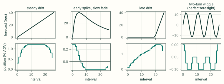
The naive rule loses money on every shape with an edge. It pays for two full-size impact events against a forecast it only partly captures. The optimal path earns money on the same forecasts because it:
- sizes to the edge;
- spreads its trading across the day's liquidity;
- exits before the forecast peaks, because the last few basis points of a flattening curve are not worth the cost of trading around the top;
- and, where allowed, trades the fade.
If short selling is banned, the spike forecast earns $46 instead of $50: the path goes long early and is flat again within the first third of the session.
The wiggle row needs its label. The optimiser was told the turning points in advance, so its $16 is what a perfect forecast of the wiggles would be worth, net of costs. Even with perfect foresight, the edge nearly all goes on costs. The next section shows what happens when that forecast is merely overconfident.
Risk aversion changes when, not just how much
The late-drift forecast puts all of its expected return in the last quarter of the day. A risk-neutral optimiser starts building from the open, because spreading purchases across more intervals lowers impact, and holding inventory costs it nothing. Adding a penalty on inventory changes that. But it is worth checking whether the penalty only shrinks the position or also changes the timing.
We compared each risk-averse path with a risk-neutral path capped at the same peak size:
| Inventory penalty | Peak position (% of daily volume) | Share of peak held before the drift arrives | Same peak, risk-neutral | Net |
|---|---|---|---|---|
| 0 | 1.60 | 92% | 92% | +$302 |
| 0.1 | 0.45 | 72% | 94% | +$153 |
| 0.5 | 0.15 | 50% | 100% | +$62 |
| 2.0 | 0.05 | 0% | 100% | +$22 |
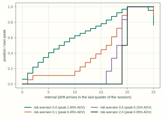
At the same peak size, a risk-neutral trader would still build the whole position before the drift arrives. The risk-averse trader waits: at the highest penalty it does not start until the interval in which the drift begins. Risk aversion delays entry as well as shrinking it, which is Almgren and Chriss's trade-off at work.
Overconfidence is expensive; underconfidence is cheap
The closed form above covers a single trade. The same test on paths: the optimiser plans on a forecast whose amplitude is scaled up or down, and the path it chooses is then scored against the true curve.
| Forecast shape | Plan on ½× | 1× (true) | 1.5× | 2× | 3× |
|---|---|---|---|---|---|
| Steady drift | +$41 | +$196 | −$230 | −$919* | −$1,126* |
| Late drift | +$65 | +$302 | −$304 | −$516* | −$629* |
| Early spike, slow fade | +$9 | +$50 | −$93 | −$711 | −$4,550 |
| Two-turn wiggle | $0 | +$16 | −$56 | −$391 | −$2,534 |
* The plan hit the 5%-of-daily-volume position limit of the toy, so these losses are lower bounds: an unconstrained optimiser would size larger and lose more.
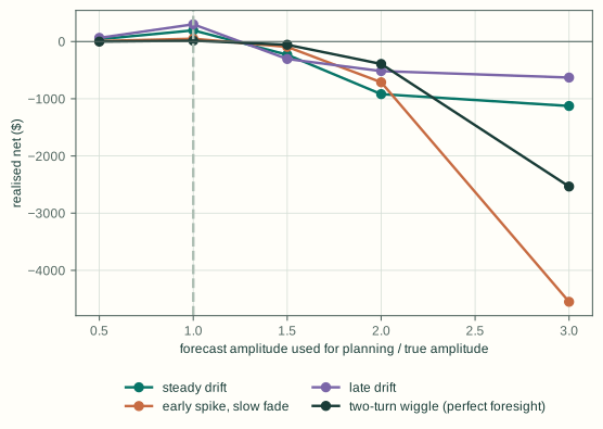
Every shape turns loss-making by 1.5× — right where the one-trade formula puts the break-even under square-root impact. The optimiser pays certain costs to chase an edge that is not there. Oversized steady positions pay impact they cannot earn back. Forecasts with turns add round trips on top: a spike forecast overstated by 3× loses about ninety times what the true forecast earns. Understating any forecast by half, by contrast, gives up at most a few hundred dollars.
Timing errors behave more gently. Planning on a spike that turns twice as early as the truth still earns $18; one that turns twice as late earns $34, against $50 with the correct timing.
The conclusion is not subtle: shrink forecasts toward zero before they reach an optimiser. A forecast used for execution should be judged by the decisions it produces, not only by its average error. When in doubt, under-state it: the cost is bounded, while the cost of over-stating it is not.
How much is the closing auction worth?
In the one-trade formula, an impact-free exit multiplies optimal size by four. In the path problem the effect is smaller, because the optimiser adapts: when the close is thin, it exits earlier through continuous trading.
Cutting the closing event from 11% to 3% to 1% of daily volume shrinks the steady-drift position from 1.2% to 0.98% to 0.90% of daily volume. Net profit falls from $196 to $153 to $140. A deep close is valuable, but a good path substitutes around a thin one.
Exit liquidity has also been growing where passive money trades. Bogousslavsky and Muravyev (2023) report that the US closing auction's share of daily dollar volume rose from 3.11% in 2010 to 7.48% in 2018.
Where implementation value is won
Clarke, de Silva and Thorley (2002) extended the fundamental law of active management to IR ≈ TC × IC × √Breadth. The transfer coefficient TC measures how faithfully the portfolio expresses the forecasts. Constraints, costs and crude trading rules lower it. The path from forecast to position is where the transfer coefficient is won or lost.
The corresponding measurement is implementation shortfall (Perold 1988). Measured against the forecast path you meant to follow, not only against the arrival price, it shows how much of the forecast actually reached the portfolio.
What the toy leaves out
- Impact that persists and decays between intervals (Obizhaeva and Wang), which couples decisions across time.
- Re-planning as the forecast updates during the day. Our paths are planned once, against a known curve.
- Execution uncertainty: fill risk, adverse selection on passive orders, and imbalance risk in auctions.
- Portfolio effects: cross-asset risk, borrow availability and cost, financing and risk budgets.
- Calibration: every cost and liquidity constant here is invented, so the dollar figures only illustrate the direction of each effect.
Takeaways
- Ask for the curve, not the sign. When the return arrives determines how to trade it.
- Expect to keep about a third of the after-spread edge at the right size under square-root impact, three-eighths at the 3/5 exponent. A backtest that keeps much more is probably using a cost model that is too kind.
- Price the exit before the entry. An impact-free exit multiplies optimal size by 2^(1/β).
- Shrink forecasts before optimising. Sizing on more than (1+β)× the true edge loses money: 1.5× under the square-root law.
- Let "do nothing" win when the edge sits inside the cost band.
References
- Almgren, R., and Chriss, N. (2000). Optimal execution of portfolio transactions. Journal of Risk 3(2), 5–39.
- Almgren, R., Thum, C., Hauptmann, E., and Li, H. (2005). Direct estimation of equity market impact. Risk, July.
- Bertsimas, D., and Lo, A. W. (1998). Optimal control of execution costs. Journal of Financial Markets 1(1), 1–50.
- Bogousslavsky, V., and Muravyev, D. (2023). Who trades at the close? Implications for price discovery and liquidity. Journal of Financial Markets 66, 100852.
- Boyd, S., Busseti, E., Diamond, S., Kahn, R. N., Koh, K., Nystrup, P., and Speth, J. (2017). Multi-period trading via convex optimization. Foundations and Trends in Optimization 3(1), 1–76.
- Clarke, R., de Silva, H., and Thorley, S. (2002). Portfolio constraints and the fundamental law of active management. Financial Analysts Journal 58(5), 48–66.
- Davis, M. H. A., and Norman, A. R. (1990). Portfolio selection with transaction costs. Mathematics of Operations Research 15(4), 676–713.
- Gârleanu, N., and Pedersen, L. H. (2013). Dynamic trading with predictable returns and transaction costs. Journal of Finance 68(6), 2309–2340.
- Gatheral, J. (2010). No-dynamic-arbitrage and market impact. Quantitative Finance 10(7), 749–759.
- Lehalle, C.-A., and Neuman, E. (2019). Incorporating signals into optimal trading. Finance and Stochastics 23, 275–311.
- Obizhaeva, A. A., and Wang, J. (2013). Optimal trading strategy and supply/demand dynamics. Journal of Financial Markets 16(1), 1–32.
- Perold, A. F. (1988). The implementation shortfall: paper versus reality. Journal of Portfolio Management 14(3), 4–9.
- Tóth, B., Lempérière, Y., Deremble, C., de Lataillade, J., Kockelkoren, J., and Bouchaud, J.-P. (2011). Anomalous price impact and the critical nature of liquidity in financial markets. Physical Review X 1, 021006.