
Who Has to Trade? Finding Alpha in Other People's Constraints
Investors who must trade leave predictable footprints. Three simulations show how the obvious measurements misread them, why competing anticipators can erase the reversal studies look for, and a one-page card that prevents both mistakes.
In 1986 two papers showed that a stock's price jumps when Standard & Poor's announces it will join the S&P 500, by roughly 3%, even though nothing about the company has changed (Shleifer 1986; Harris and Gurel 1986). It became the textbook demonstration that demand curves for stocks slope down. Index funds had to buy, so the price had to rise until someone was willing to sell to them.
The effect then grew with the index industry. In the working-paper version of their study, Greenwood and Sammon measure the average abnormal return of an addition, from the day before the announcement to the day after the stock enters the index, at about 7% in the 1990s. By 2010–2020 it had fallen to 0.8%, statistically indistinguishable from zero. Deletions followed the same path, to −0.6%.
This was not because index funds stopped buying. Over the same period, buying by S&P 500 trackers rose from close to zero to more than 6% of an added company's shares. The price response per unit of net forced demand — Greenwood and Sammon's "multiplier" — fell from about 6.8 in the late 1990s to about 0.4 in the 2010s.
The forced buyers did not change. What changed was who else knew they were coming, and who was set up to sell to them.
That is the whole article in miniature. A trader who must trade leaves a footprint you can predict. The footprint is worth something only to whoever is paid to absorb it. And measuring it correctly is harder than it looks.
Start from a constraint, not a correlation
Most alpha research starts from a pattern: a variable that predicted returns in a backtest. We start from a person with a problem. Someone has a mandate, a redemption, a margin call or a tax position that forces them to trade regardless of price. A binding constraint makes a hypothesis unusually specific. Before touching any data, it tells you five things:
- Sign. Which way the forced trader must trade.
- Timing. When the trade must happen, and when others can know about it.
- Dose. How large the trade is relative to the liquidity available to absorb it.
- Heterogeneity. Where the effect should be larger: thinner stocks, scarcer arbitrage capital, fewer offsetting flows.
- Reversal. Whether the price effect should unwind once the forced trade is done. Temporary pressure unwinds; information does not. As we show later, this prediction only holds if few others are competing to absorb the trade.
Five predictions made in advance are what separate a mechanism from a story told after the fact. If the effect appears with the wrong timing, does not scale with the dose, or fails to reverse where few others could have absorbed the trade, the hypothesis is in trouble. Hypotheses built from correlations rarely offer that many ways to be wrong.
The literature is full of constrained traders:
| Who | Constraint | Predicted footprint | Evidence |
|---|---|---|---|
| Index trackers | Must hold the published index | Buying at known dates, scaled by weight change relative to liquidity; later reversal | S&P 500 inclusions (Shleifer 1986; Harris and Gurel 1986); Nikkei 225 redefinition (Greenwood 2005) |
| Open-end funds with redemptions | Must raise cash | Pro-rata selling of existing holdings; pressure in stocks held in common | Coval and Stafford (2007) |
| Leveraged traders | Margin and risk limits | Selling into declines; others trade ahead; price overshoots then recovers | Brunnermeier and Pedersen (2005) |
| Aggregate institutional money | Near-fixed equity allocations | Small net flows move aggregate prices a lot | Gabaix and Koijen (2021): about $5 of market value per $1 of net flow |
Greenwood's Nikkei study is the cleanest illustration of what "absorbing" a forced trade involves. In April 2000, Nikkei replaced 30 of the 225 stocks in its index, and about ¥2.4 trillion of tracking money had one week to rebalance. The deleted stocks fell about 30% that week and the added stocks rose about 19%. Then the prices came back. About a third of the event return reversed in the following week, more than half within five weeks, and all of it within ten.
Those who sold to the index funds were paid, but not for free. Greenwood estimates that an arbitrageur absorbing just 1% of the demand would have been down ¥4.17 billion at the worst point, and did not recover the loss until November. The return to liquidity provision is compensation for carrying that risk.
Draw the graph before you query the data
The data will not tell you which variables to control for. The mechanism will. Before running any regression, we write down the causal graph. For forced fund flows it looks like this:
- A constraint shock (investors redeem from a fund) causes forced trading in the fund's existing holdings.
- Forced trading moves the price today, and part of that move reverses later.
- Separately, news about a company moves its price directly, and prompts informed trading that moves the price the same way.
- There is a back door: news about a fund's biggest holdings affects the fund's performance, which affects redemptions. The forced flow is not independent of the news it will be confused with.
Two lessons follow before any data arrives. First, observed net trading mixes forced and informed demand, so it cannot be treated as the forced component. Second, some tempting controls make things worse. Controlling for same-period volume or same-period return conditions on variables that are caused by the flows being studied. Cinelli, Forney and Pearl (2024) call these bad controls.
López de Prado (2023) names the resulting failure well. Some findings are spurious because of chance and data mining. Others are statistically real but causally misread. The rest of this article is about the second kind.
Demonstration 1: observed flow is not forced flow
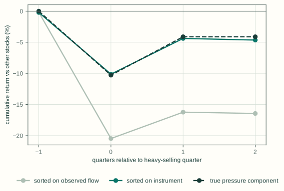
To make this concrete we built a synthetic market in which we know the truth. There are 400 stocks, 40 quarters and 60 funds. Each fund holds 40 stocks. Every quarter, investors add to or redeem from each fund, occasionally in large waves, and funds trade their existing holdings in proportion.
Forced trading moves prices by exactly 2% for every 1% of a company's shares traded, and 60% of that move reverses the next quarter. Stock news moves prices permanently, and informed traders trade in the direction of the news. We simulated the market 200 times.
A researcher who only sees total net trading, and regresses returns on it, finds:
| What is estimated | Truth | Naive regression on observed flow | Regression using a clean instrument |
|---|---|---|---|
| Price effect in the trading quarter | 2.00 | 2.94 | 1.98 |
| Price change the next quarter | −1.20 | −0.60 | −1.16 |
| Share of the effect that reverses | 60% | 20% | 59% |
Means across 200 simulated markets. The 5–95% ranges are narrow: naive 2.88–2.99 and −0.66 to −0.54; instrument 1.91–2.04 and −1.26 to −1.06. Standard errors are clustered by quarter.
The naive researcher does not fail to find an effect; they find the wrong one. Observed flow includes informed trading, which is correlated with news that does not reverse. So the price effect looks 47% too large, the reversal looks half as big, and the implied reversal share is 20%. The natural conclusion is that "these flows are mostly informed". That is exactly backwards: in this market, 60% of the effect is temporary price pressure, a liquidity premium someone could earn.
The algebra is short enough to state. Write observed flow as forced flow plus informed trading, O = F + bN. The naive same-quarter slope converges to (λ·Var F + b·Var N)/Var O, which is inflated by the informed term. The naive next-quarter slope is the true reversal multiplied by Var F/Var O, which is 0.5 in our simulated market.
The fix uses the mechanism. A fund's holdings at the start of the quarter are known before the quarter's news arrives. Fund-level flows are driven by fund-level investor behaviour. Multiplying one by the other gives the trade each stock should experience mechanically: a "flow-to-stock" instrument that owes nothing to the stock's own news. Using it recovers both the impact and the reversal.
One further lesson from the same simulation. The instrument varies at the level of fund flows, which hit many stocks in the same quarter at once. Stock-quarters are therefore not independent observations. A placebo test — regressing last quarter's return on this quarter's instrument, where the truth is zero — rejects the null 21% of the time with standard heteroskedasticity-robust errors, instead of the nominal 5%. With errors clustered by quarter it rejects 7% of the time. Choosing the right unit of observation is not a technicality. It separates a finding from an artefact.
Demonstration 2: a measure that contains its own answer
The first demonstration had a clean instrument available. The second shows how an instrument can look clean and not be.
A large literature measures fund "fire-sale" pressure by estimating how much redeeming funds must sell of each stock, and dividing by the stock's dollar trading volume that quarter. Wardlaw (2020) pointed out the flaw. The holdings being sold are valued at the start-of-quarter price, but dollar volume is measured at during-quarter prices. The ratio therefore contains, roughly, one divided by one plus the stock's own return that quarter. A stock that fell looks more "pressured" by construction. The measure is, in Wardlaw's words, "inadvertently a direct function of a stock's actual realized return during the outflow quarter".
To see how much damage this does, we reran our synthetic market with no price pressure at all: forced trading has zero effect on prices. We then sorted stocks each quarter on three versions of outflow pressure and compared the most-pressured decile with the rest.
| Pressure measure | Same-quarter return, most-pressured decile vs rest | Next-quarter return | How often the null is rejected (same / next) |
|---|---|---|---|
| Shares to be sold ÷ shares outstanding | +0.02% | +0.02% | 5% / 4% |
| Shares to be sold ÷ last quarter's volume | −0.00% | +0.01% | 6% / 2% |
| Dollar value to be sold ÷ this quarter's dollar volume | −4.71% | +0.97% | 100% / 70% |
200 simulated markets; t-statistics from the quarterly time series of decile spreads.
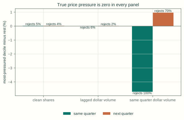
The contaminated measure manufactures a complete fire-sale story from nothing. The pressured stocks fall 4.7% (t ≈ −13, significant in every simulation) and recover about a fifth of that the following quarter (significant 70% of the time). The "recovery" comes from ordinary short-term price noise that happens to be selected by a sort which is itself selecting on returns. The two clean versions find nothing, as they should.
The rule we take from this is simple and strict. A treatment variable must be computable from information dated before the outcome window, and must never be scaled by a quantity measured inside it. Volume, price and volatility from the same period are the usual offenders.
Natural experiments are not free
When an index uses a mechanical rule — the largest 1,000 stocks go in one index and the next 2,000 in another — firms just either side of the cutoff look like a natural experiment. Chang, Hong and Liskovich (2015) use the Russell 1000/2000 boundary this way to measure the price effect of index assignment.
The design is powerful, and it is easy to implement incorrectly. Wei and Young (2024) show that under the most common implementation of the Russell cutoff, institutional ownership measured before reconstitution already differs at the cutoff. Differences attributed to index assignment are then partly selection.
The general lesson: reconstruct the assignment rule exactly as the index provider applies it. Before interpreting any post-event outcome, test that pre-event outcomes do not already jump at the threshold.
When everyone knows who has to trade
A forced trade that is predictable invites anticipation. Brunnermeier and Pedersen (2005) show that when a large trader must sell, others may sell ahead of them and buy back later. The price overshoots, and the forced seller receives less. Duffie (2010) describes the other half of the dynamic: capital that could absorb a shock arrives slowly, so the initial impact is sharp and the recovery gradual. The recovery speeds up as capital and attention move in.
Greenwood and Sammon's post-mortem of the S&P 500 index effect shows the market adapting:
- Netting. In their words, migrations from the S&P MidCap index "went from about 50% of additions to over 70%", and the trend was even stronger among deletions. For those stocks, MidCap funds were selling as S&P 500 funds were buying.
- Market adaptation. Beyond netting, the market became far better at providing liquidity to index changes, with dedicated trading desks and pre-announced rebalancing schedules.
So which is it? Do traders who see a forced trade coming prey on it, as in Brunnermeier and Pedersen, or absorb it and make it cheaper, as the index-effect history suggests? A recent paper answers that the same behaviour can do either, and says what decides it.
A game among the anticipators
Fiechtner and Blanchet (2026) model an index reconstitution as a game. An index fund must rebalance and, once the new membership is announced, follows a fixed execution schedule ending on the implementation date; a short window stands in for the closing auction. A group of "opportunists" can position before the announcement, revise after it, and trade against the fund while it executes. Prices carry transient impact that decays over time, and — the crucial modelling choice in their baseline specification — opposing buy and sell flows offset in the price everyone pays. The authors solve for a subgame-perfect equilibrium in which each trader reacts to the market as it evolves. Their numerical illustrations are meant, in their words, to "showcase the qualitative properties of the model" rather than to fit real rebalances.
Four findings matter for anyone studying forced traders:
- Competition hands the premium to the forced trader. As the number of opportunists grows, "both mean and total wealth decline… more opportunists offset a larger fraction of the fixed indexer orders, reducing the price displacement from which the group profits." The index fund's savings rise, mostly as the first few competitors arrive.
- Crowds overshoot; a monopolist does not. With many opportunists, the group's position in each added or deleted stock "passes through zero" while the fund is trading: in aggregate they sell more than they held, then cover. With a single opportunist "there is no crossing through zero". The authors note that this matches the rise and subsequent fall in short interest that Pegoraro, Sammon and Shim document for S&P 500 additions from outside the index family.
- The sign depends on competition and how fast impact decays. In the authors' summary, their illustrations "show how competition and impact decay determine whether anticipatory trading raises or lowers the indexer's execution costs". "With slow decay, adverse impact from opportunists' earlier trades persists into implementation and can outweigh the benefits of their opposing trades." Savings peak at intermediate decay: when impact decays very fast, the fund's own impact fades quickly too, leaving less to offset.
- Agreement moves prices; disagreement moves volume. The equilibrium "separates the effects of average membership beliefs on aggregate inventories and price impact from the effects of disagreement on individual positions". Disagreement "generates substantial additional gross trading volume" that cancels in aggregate. Heavy trading around an event is therefore not, by itself, evidence of heavy net pressure.
Bessembinder, Carrion, Tuttle and Venkataraman (2016) reach the same conclusion from a simpler model of a predictable liquidation, and provide related evidence: even a monopolist improves market quality "if trades' temporary price impacts are quickly reversed", and "competition among strategic traders strictly improves market quality".
This is a different route to the erosion Greenwood and Sammon measured, not the same one. In the model, anticipators absorb a single fund's fixed order. Migrations net one index fund's buying against another fund's selling, which the model leaves out (it could be added by treating the order as the net flow of all affected funds). Two independent routes to a smaller price response make the decline harder to explain away, not easier.
Predation and liquidity provision are therefore not two different kinds of trader. They are the same behaviour under different market conditions.
Demonstration 3: what a crowd of anticipators does to the evidence
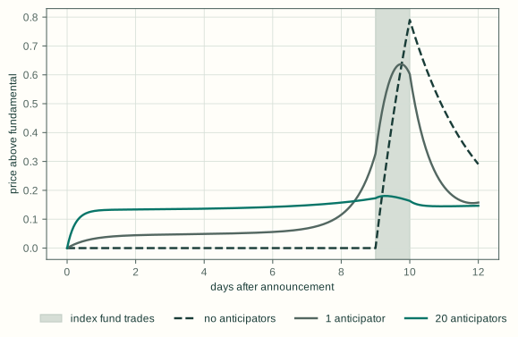
To see what this means for measurement, we built a deliberately stripped-down version of the game:
- Setup. One stock. An index fund must buy a fixed quantity, spread evenly over one day that starts nine days after the announcement. Trading continues for two days afterwards.
- Traders. Some number of identical anticipators start and finish flat, pay a small penalty for holding inventory, and choose their trades knowing the fund's order.
- Prices. Price impact decays exponentially (half-life about 1.4 days in the baseline). Every trader pays the same price, which rises with the net of all flows.
- Solution. We solve for the equilibrium in which each anticipator plans a path given everyone else's (an open-loop equilibrium, simpler than the paper's). All figures are relative to what the fund would pay with no anticipators.
| Anticipators | Index fund's cost | Anticipators' total profit | Their net position when the fund finishes | Price displacement: when the fund finishes → two days later |
|---|---|---|---|---|
| none | 100% | — | — | 0.79 → 0.29 |
| 1 | about unchanged | 40% | long 0.18 | 0.60 → 0.16 |
| 3 | 57% | 25% | short 0.02 | 0.30 → 0.15 |
| 20 | 29% | 4.8% | short 0.13 | 0.16 → 0.15 |
| 50 | 26% | 2.0% | short 0.14 | 0.15 → 0.15 |
Positions are fractions of the fund's order; price displacement is in units of impact per unit of that order. The simulation is solved at 64 time steps a day; every sign in this section is unchanged at 32.
Three things happen as the crowd grows.
The premium moves to the forced trader. One anticipator earns 40% of what the fund would otherwise have paid. Twenty earn 4.8% between them, a quarter of a percent each. The fund's cost falls by 71%. The liquidity became cheap because it became competitive.
The price moves earlier, and the reversal disappears. Without anticipators, the price stays flat until the fund starts buying, rises to 0.79 while it trades, then gives back nearly two-thirds within two days. With twenty anticipators, it reaches 0.13 within a day of the announcement — four-fifths of where it will be when the fund finishes — and falls only from 0.16 to 0.15 afterwards. The forced buyer is still there, still buying the same quantity. But a study that looks for a price move around the execution date, followed by a reversal, finds almost nothing. That is prediction 5 failing while the mechanism is fully at work.
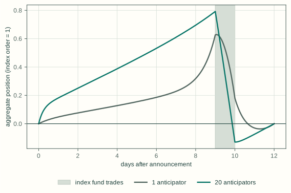
Crowds overshoot, and a lone trader does not. A single anticipator sells into the fund's buying but is still long when the fund finishes. Twenty anticipators together sell more than they held and are net short by 13% of the fund's order, then buy back afterwards. That buying-back is part of why the price does not fall afterwards.
How quickly impact decays decides whether anticipation helps or hurts the forced trader:
| Impact decay (per day) | Fund's cost change, 20 anticipators | Fund's cost change, 1 anticipator |
|---|---|---|
| 0.01 (nearly permanent) | +26% | +244% |
| 0.1 | −31% | +103% |
| 0.3 | −62% | +29% |
| 1 | −79% | −20% |
| 10 | −86% | −42% |
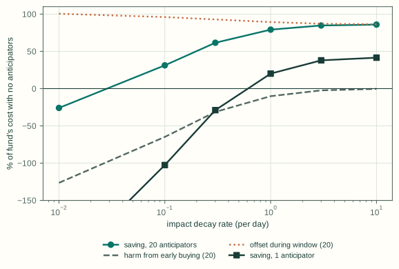
The +244% corner needs two conditions at once: impact that barely decays, and a lone anticipator free to build a position more than twice the size of the fund's entire order before the fund starts trading.
When impact barely decays, the anticipators' early buying pushes up the price the fund pays by more than their selling offsets later: the crowd preys on the fund. When impact decays in a day or two, the same buying costs the fund little and the offset dominates: the crowd provides liquidity. A lone anticipator preys unless impact decays quickly.
The crowd's harm at slow decay also depends on how expensive it is to trade quickly. Double the cost of fast trading relative to impact and twenty anticipators save the fund 4% even when impact is nearly permanent; double it again and they save 35%. A lone anticipator still raises the fund's cost in both cases (by 97% and 16%). This is the dependence Fiechtner and Blanchet report: at low resilience, opportunists "can be harmful when Λ is small relative to Γ", that is, when the cost of trading quickly is small relative to price impact. Brunnermeier and Pedersen's world and Greenwood and Sammon's world are two regions of one map.
What this changes for research
- Measure from the date the constraint becomes predictable, not the date the trade is executed. With competitive anticipation, most of the price move happens at the announcement, or before it. Fiechtner and Blanchet point out that in the published version of Greenwood and Sammon's study, abnormal returns over the 100 trading days before an S&P 500 announcement rose from 9.6% in the 1990s to 18.7% in 2010–2020. That may be anticipation, the selection of past winners, or both.
- Do not treat a missing reversal as evidence against forced trading. When the liquidity to absorb a forced trade is competitive, the reversal shrinks towards nothing while the forced trader is still paying. Test the timing of the move and its relation to net demand instead.
- Estimate net demand, including the anticipators'. Offsetting flows from other forced traders and the anticipators' own positions both change the dose. Gross volume around the event partly reflects disagreement among anticipators, which cancels in aggregate.
- Model who else is positioned, and how fast impact decays. The premium belongs to whoever absorbs the forced trade, collectively. It shrinks as they multiply, and it can turn from a cost to the forced trader into a benefit as impact decays faster.
- Treat the size of a forced-trading premium as a parameter that decays, and monitor it like one. A mechanism can be completely real and still stop paying.
The mechanism card
Every constrained-trader hypothesis we test starts from a single page, filled in before any data is queried:
- Actor and constraint. Who must trade, and what forces them?
- Trigger and timing. What starts the trade? When does it become knowable, and to whom?
- Dose. Expected forced quantity relative to expected liquidity over the window.
- Predictions. Sign, horizon and expected reversal fraction — given how many others are likely to be positioned for the same trade.
- Competition and resilience. Who else can see the constraint, when, and how quickly impact decays in this market. These decide whether anticipators prey on the forced trader or supply its liquidity, and whether a reversal should be visible at all.
- Heterogeneity. Where the effect should be stronger, and why.
- Treatment construction. Show that every input is dated before the outcome window, with none scaled by an outcome-window quantity.
- Unit of observation. The level at which the treatment varies, which is the level at which errors are clustered.
- Placebos. Pre-period returns, stocks the forced trader does not hold, and shuffled event dates.
- Competing explanations. For each one, the test that separates it from the mechanism.
- Kill criteria. Which results would make us drop the idea?
A hypothesis that cannot fill in this page is not ready for a backtest.
What this does not show
The three simulations show how common estimators and a simple strategic market behave under stated assumptions, with every parameter set by us. The anticipation game is a toy: one stock, an order known from the start, identical traders, and a simpler equilibrium concept than Fiechtner and Blanchet's. Their own illustrations are stylised too: five stocks, traders who start flat, strong penalties for ending with inventory, constant fundamental prices, the closing auction approximated as continuous trading, and no borrowing costs. None of this measures the size of any real forced-trading effect, or shows that any particular constraint is tradable after costs today. The index-effect history suggests many are not.
The claim is narrower and, we think, more useful. When the data are generated by a constrained trader, the obvious measurements can point confidently in the wrong direction. Starting from the constraint is what lets you design measurements that point the right way.
References
- Bessembinder, H., Carrion, A., Tuttle, L., and Venkataraman, K. (2016). Liquidity, resiliency and market quality around predictable trades: theory and evidence. Journal of Financial Economics 121(1), 142–166.
- Brunnermeier, M. K., and Pedersen, L. H. (2005). Predatory trading. Journal of Finance 60(4), 1825–1863.
- Chang, Y.-C., Hong, H., and Liskovich, I. (2015). Regression discontinuity and the price effects of stock market indexing. Review of Financial Studies 28(1), 212–246.
- Cinelli, C., Forney, A., and Pearl, J. (2024). A crash course in good and bad controls. Sociological Methods & Research 53(3), 1071–1104.
- Coval, J., and Stafford, E. (2007). Asset fire sales (and purchases) in equity markets. Journal of Financial Economics 86(2), 479–512.
- Duffie, D. (2010). Presidential address: asset price dynamics with slow-moving capital. Journal of Finance 65(4), 1237–1267.
- Fiechtner, L.-B., and Blanchet, J. (2026). Strategic index reconstitution: differential games, closed-loop equilibria and mean-field dynamics. arXiv:2609.15901.
- Gabaix, X., and Koijen, R. S. J. (2021). In search of the origins of financial fluctuations: the inelastic markets hypothesis. NBER Working Paper 28967.
- Greenwood, R. (2005). Short- and long-term demand curves for stocks: theory and evidence on the dynamics of arbitrage. Journal of Financial Economics 75(3), 607–649. Figures quoted here are from the working-paper version.
- Greenwood, R., and Sammon, M. (2022). The disappearing index effect. NBER Working Paper 30748. Published in Journal of Finance 80(2), 657–698 (2025). Figures quoted here are from the working-paper version, except the 100-day pre-announcement returns, which are from the published version as reported by Fiechtner and Blanchet.
- Harris, L., and Gurel, E. (1986). Price and volume effects associated with changes in the S&P 500 list: new evidence for the existence of price pressures. Journal of Finance 41(4), 815–829.
- López de Prado, M. (2023). Causal Factor Investing: Can Factor Investing Become Scientific? Cambridge University Press.
- Pegoraro, S., Sammon, M., and Shim, J. J. (2026). Optimal index-linked rebalancing with anticipatory trading. Working paper, SSRN 6772502. Cited as described by Fiechtner and Blanchet.
- Shleifer, A. (1986). Do demand curves for stocks slope down? Journal of Finance 41(3), 579–590.
- Wardlaw, M. (2020). Measuring mutual fund flow pressure as shock to stock returns. Journal of Finance 75(6), 3221–3243.
- Wei, W., and Young, A. (2024). Selection bias or treatment effect? A re-examination of Russell 1000/2000 index reconstitution. Critical Finance Review 13(1–2), 83–115.